Introduction to Six Sigma

Like many quality professionals, I’ve seen scores of quality methods come and go over the years. Most methods generate hype initially, but their use tends to wane as reports surface on failures to realize operational and business gains. Then the inevitable controversy and debate begins. Professionals and organizations ask: Why did that happen? Whose fault is it? Is the organization or method to blame?

Six Sigma received a high degree of attention in the mid-1980s when it was first introduced by Motorola.¹ In 1988, Motorola received the prestigious Baldrige National Quality Award from the United States. The award recipient profile for Motorola states: “to accomplish its quality and total customer satisfaction goals, Motorola concentrates on several key operational initiatives. At the top of the list is Six Sigma quality."²

The Six Sigma (SS) approach rose to fame in the business world in the late 1990s after General Electric CEO Jack Welch shared the breakthrough business gains the organization experienced a result of implementing a SS program.

Organizations from all over the world from all sectors—manufacturing, service, education, healthcare, government, logistics and supply chain—began to use SS. Of course, not all organizations that that endeavored to use SS realized the dramatic gains reported by General Electric and Motorola. As is the case with most quality methods, failure is usually related to leadership and culture structure that is not ready to accept the approach.

SS is different from other quality improvement methods. It’s technical and is packaged into a well-defined systematic improvement cycle known as define, measure, analyze, improve and control. This brings joy to a quality professional like myself who recognizes the value of statistics and technical quality tools (including statistical quality control, regression analysis, hypothesis testing, inspection plans and others).

But if you’re not a statistician, you might experience difficulty understanding SS. In this article, I’ve provided a simplified view of the technical aspects included in the SS method. Specifically, I focus on the meaning of Sigma and how it relates to the SS method.

What is Sigma?
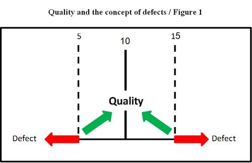
Let’s assume that we have a laboratory process which requires that tests be performed at temperatures of 10±5 ºC. Therefore, the specification limits are five and 15—where five is the lower specification limit (LSL) and 15 is the upper specification limit (USL). Our nominal or target value (TV) is 10.

The closer the test performance is to the TV, the better the quality of the result. If the test performance is to the left of LSL or to the right of USL, the test result is classified as bad—it means there is a defect. This concept is illustrated in Figure 1.

Let’s assume that lab A and lab B perform the same test. Table 1 shows the results for seven tests conducted at each lab.

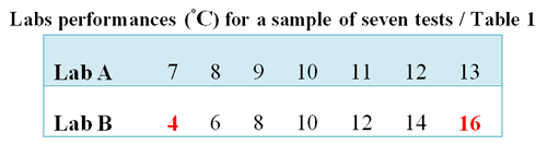
Table 1 shows lab A has no defects—all values are within specification limits. Lab B has two defects—four and 16. On average (denoted by the symbol ), both labs have the same performance of 10 (which is right on the TV). The sample average is calculated using the following formula:

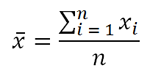
where  refers to individual temperature values and n to total number of values in the sample (i.e. seven).

However, lab B has more variation (spread of data) than lab A. Note that in lab A, the difference between consecutive values is one and two for the values of lab B. To capture that property of variation, we use sample standard deviation (s) as an estimate of the population standard deviation Sigma, which has the following formula:

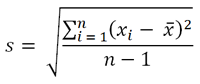
As expected, the s of lab B is 4.32, which is twice of that of lab A (2.16). The  and s for a given sample may be determined using the Excel functions of “AVERAGE” and “STDEV.”

We conclude this section with a clear answer to our question: What is Sigma? Sigma is a measure of data variation or process variation. The closer data (coming off a process) is to each other, the lower the s (assumed estimate of Sigma) is (as in lab A), the higher the precision, and the better the quality. A key challenge for quality professionals is to improve the process by reducing the value Sigma.

Graphical Meaning of Sigma
Continuing with our lab example, let’s assume that we take larger samples from each lab and obtain the results shown in Tables 2 and 3. Note that we have intentionally maintained the original mean and variation levels for the two labs..

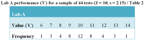
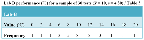
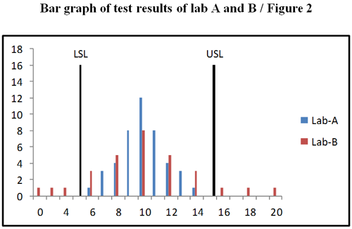
We may represent the data in Lab-A and Lab-B using a bar graph as shown in Figure 2. It is clear that lab B has more variation (s) than lab A, which leads to more defects (values to the left of LSL and to the right of USL).

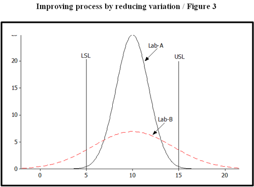
A continuous line chart is often used for representation as shown in Figure 3. The pattern shown in Figure 3 is called a normal pattern or distribution. The normal distribution is commonly found to represent many real-world processes. We can see that we must reduce variation of the process in order to improve performance. Reducing process variation is at the heart of SS.

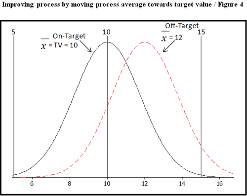
Another recommendation would be to move the process average, estimated by , to align with TV. For example, if the lab-A process average  is off-target, we should improve the process by moving it on-target TV as shown in Figure 4.

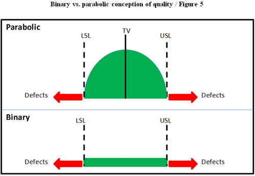
Many organizations have a binary perspective on output performance of the process (either inside or outside specification limits), so a test result value that is barely within specification (say, 4.9 as in our example) is considered to be as good as a test result that is close to the TV (say, 10.5). Figure (5) illustrates the binary and parabolic concepts of quality.

Sigma and Six Sigma Riddle
It is logical to conclude that a process with higher Sigma yields more defects. However, paradoxically, a SS process yields less defects than a three, four or five Sigma processes. In this section, we will examine another example.

The Sigma in the SS method refers to the distances of LSL and USL from the TV; where the natural tolerance of the process is ±3s and the process mean (m) is either on TV or is allowed to shift by ±1.5s, as recommended by Motorola and the majority of SS practitioners (see Figure 6). It is important to note that both population standard deviation s and population process mean m are usually unknown in real applications; and therefore need to be assumed. We make such an assumption in the remainder of the article.

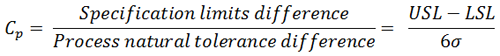
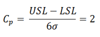
The main driver of SS is to reduce process variation, represented by Sigma, so the process average of the natural tolerance process is at least SS away from the specification limits on both sides, resulting in a process capability ratio Cp of two as calculated by the following formula:

So, for a SS performance:

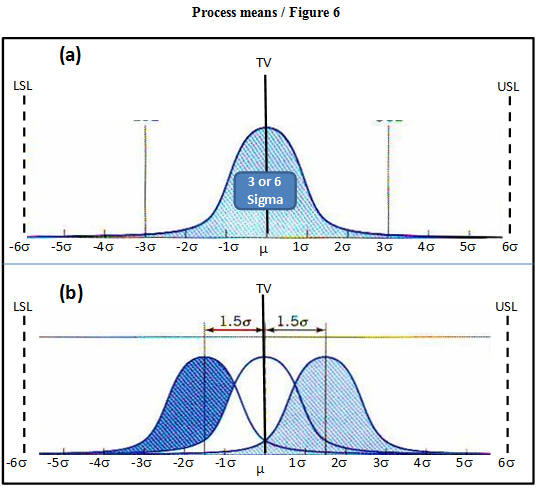
Under graph, include note: The SS processes with a process average m on TV is depicted in Figure 6a. The process average m shift off TV by ±1.5s is depicted in Figure 6b.

Table 4 compares the performance for both cases of the SS concept. For the case where process mean m is on TV, the SS performance is two defective parts per billion (ppb) whereas the SS performance is 3.4 defective parts per million (ppm) for the case where the mean m may have a ±1.5s shift.

The calculation of these results is possible using the normal distribution function. For our lab example – assuming known population mean and standard deviation – with specification limits of 10±5 ºC, one may compute the defects rate for the case of process mean on TV = 10 and s = 5 / 6 (calculated from 6s = USL – TV = 5) using the normal distribution function in Excel “NORMDIST (x, mean, sigma, 1)” as follows:

• Defect rate = 1 – P (5 < temperature < 15)

    = 1 – [NORMDIST (15,10, 5 / 6, 1) – NORMDIST(15, 10, 5 / 6, 1)] » 2 x 10-9

    = 2 ppb

If a 1.5s shift is allowed, then 1.5s = 1.5*5 / 6 = 1.25; so a 1.5s shift moves the process average  from 10 to 11.25. Therefore:

• Defects rate = 1 – P ( 5 < temperature < 15)

    = 1 – [NORMDIST(15, 11.25, 5 / 6,1) – NORMDIST(15, 11.25, 5 / 6,1)] » 3.4x10-6 = 3.4 ppm

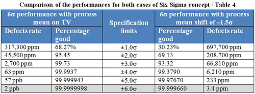
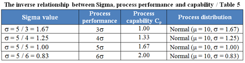
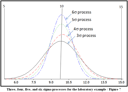
Table 5 and Figure 7 provide further resolution of the riddle involving the relationship between Sigma, process performance and capability using data from the laboratory example. The associated, assumed process distributions in Table 5 are used to construct Figure 7.

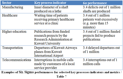
The challenge of the SS method is to utilize a set of quality and management tools in systematic way to improve key operational and business processes so they achieve SS performances for key process indicators or metrics. Table 6 provides examples of SS performances for selected processes.

According to authors Mikel Harry and Richard Schroeder, each Sigma improvement in a business process (such as moving from five sigma to SS) translates into approximately a 10% net income improvement, a 20% margin improvement and a 10 to 30% capital reduction.³ This is supported with several success stories, such as:

• By 1998, AlliedSignal saved $1.5 billion from implementing its SS program in 1994.
• By 1998, GE realized the following gains after implementing SS in 1996:
• Revenue increased 11%.
• Earnings increased 13%.
• Working capital turns increased to 9.2% from 7.2%.

Conclusion
Understanding the concept of SS and how it translates into a defect rate of 3.4 ppm is at the heart of the SS method, but this is not the whole story of SS. In order to realize the successes AlliedSignal, GE, and others enjoyed, the organization should provide for specific organization-wide measures and provisions especially at the levels of qualifying intellectual capital and following a systematic process improvement method.

References

1. S.E. Blashka, J. Crager, D. Lemons, W. Vestal, “Six Sigma Management—A Guide For Your Journey to Best-Practice Processes.” APQC, 2004.
2. The National Institute of Standards and Technology, “Baldrige Performance Excellence Program,” http://www.baldrige.nist.gov/Motorola_88.htm.
3. Harry, M. and Schroeder, R. “Six Sigma–The Breakthrough Management Strategy Revolutionizing the World’s Top Corporations,” Soundview Executive Book Summaries, Vol.22 No.11, November 2000.